METHOD OF THE CORRECTED DISTANCE FOR THE VALUATION OF REAL ESTATE: A THEORETICAL PROPOSAL IN DEVELOPMENT

MÉTODO DE LA DISTANCIA CORREGIDA PARA LA VALORACIÓN DE BIENES INMUEBLES: UNA PROPUESTA TEÓRICA EN DESARROLLO

Manuel Chacón Mateos (Universidad Marítima del Caribe, Catia La Mar, La Guaira, Venezuela)¹

Abstract

This article presents a novel valuation model by market comparison that requires a minimum application of criteria by the appraiser, thus seeking the highest degree of objectivity possible. The premise that supports the model is that the price differences observed between comparable assets of the same market must be proportional to the dissimilarities (distances) between those same assets, but it shows that not every distance implies a price gap, so a corrected distance is used. As a validation, the results of applying the method to a fictitious case, as well as to two real data sets from the commune of Providencia, in the city of Santiago, Chile, are evaluated. The solution of the model requires the use of non-linear programming, and the examples show that the results are very similar to those obtained by applying Goal Programming, which is another optimization method applicable to the valuation of real estate.

Keywords: appraisal, real estate, property valuation, applied optimization methods.

JEL Codes: C61, D46, R21, R31

Resumen

En este artículo se presenta un nuevo modelo de valoración por comparación de mercado que requiere una mínima aplicación de criterios por parte del tasador, buscando así el mayor grado de objetividad posible. La premisa que sustenta el modelo es que las diferencias de precios observadas entre activos comparables de un mismo mercado, deben ser proporcionales a las disimilitudes (distancias) entre esos mismos activos, pero se muestra que no toda distancia implica una brecha de precios, por lo que se utiliza una distancia corregida. Como validación, se evalúan los resultados de la aplicación a un caso ficticio, y también a dos conjuntos reales de información de la comuna de Providencia, en la ciudad de Santiago de Chile. La solución del modelo requiere el uso de programación no lineal, y los ejemplos muestran que los resultados son muy similares a los obtenidos aplicando Programación por Metas, que es otro método de optimización aplicable a la valoración de bienes raíces.

Palabras clave: tasación, bienes raíces, valoración de propiedades, métodos de optimización aplicados.

Clasificación JEL: C61, D46, R21, R31

1. INTRODUCTION

The main methods of real estate valuation are in two major categories: capitalization methods and comparative methods (Aznar & Guijarro, 2007). The techniques are completely different between these groups, in the first case they are based on the anticipation approach, where the projected return of the asset is calculated as a present value according to a certain discount rate. It is worth saying that there is considerable uncertainty when using the capitalization approach, both because of the uncertainty of a projected cash flow and because of the high sensitivity of the results to the rate used. Its use is justified when the information of similar transactions is limited or the purpose of the property is commercial, being intended for the generation of income.

Comparative methods, on the other hand, are based on the principle of substitution, wherein the value of a good must be similar to that of others with comparable characteristics, making them theoretically interchangeable. To put it another way “when similar real estates are available in the market, the buyer will not pay more for a particular real estate than for a similar real estate” (Kucharska-Stasiak & Źróbek, 2015). This approach is commonly chosen when dealing with houses or apartments in a mature market with transactions that can serve as references. It is within this context that the technique presented in this article is situated.

A well-known concern within the area of valuations especially when making comparisons, is that the methods used have the highest possible degree of objectivity (Guijarro, 2013), which seeks to ensure that the results obtained by two appraisers tend to coincide if they use the same data, thus providing transparency to the process. However, the homologation procedure, which is usually used in the appraisals of individual assets (as opposed to the statistical methods associated with mass appraisal) and which seeks to translate differences in attributes into differences in values, is largely subjective. There are no exact formulas or measures of similarity that can be used, leading to the use of empirical criteria and formulas (Piracés, 2019).

In particular, since it is not possible to observe in the market the marginal values of the attributes of real estate, but only their aggregate effect on certain assets, the level of importance of each factor that contributes to explaining the value becomes an aspect dependent on the discretion of the appraiser.

While techniques that provide weighting coefficients with greater objectivity (statistics/mathematics), for their part, have other disadvantages associated with having to assume a particular model (functional relationship) for the connection between the data, as will be explained in the next chapter.

Thus, it is desirable and necessary to develop methods that enhance objectivity in valuations. These methods should be parsimonious, avoiding excessive assumptions, and should employ simple and straightforward logic. Additionally, they should be adaptable to working with small samples in routine appraisal tasks. The objective of this study is to contribute an additional element in this regard: a new approach to weighting variables objectively in valuation. But in addition, the proposed approach effectively deduces weights and makes value estimates, based on the differences in prices and attributes observed in the market sample (internal consistency), with an essentially novel procedure.

As a result of the research, a method has been developed that seeks the internal coherence of the data, in the sense that the distances between the referents (generated by the differences in attributes) must be related to the price differences that exist within the sample, and at the same time (and hence the distinctive detail) taking into account the fact that not all distances can be interpreted in the same way. It should also be highlighted it is not only a way of weighting variables, but it allows making consistent value estimates on properties of interest. The method has been shown to work appropriately with the input data, illustrating its application with intentional test data and also with real transaction cases.

In the rest of the article, the reader will find four additional chapters. First, a literature review related to the topic of study is presented. In the third section, the model and its justification are presented, and then its operation is shown with a simple example in the first instance and then with data from current offers and real transactions carried out on apartments in the commune of Providencia, in the city of Santiago de Chile. Finally, the work closes with the conclusions and bibliographic references.

2. LITERATURE REVIEW

The comparison of real estate with the aim of valuing a certain property of interest admits a wide variety of procedures, but in turn it can also be subdivided into two main subcategories: direct comparison and indirect comparison.

It is said that a direct comparison is made (or that a sales comparison model is used) when the appraiser adjusts the known values of reference properties according to the similarity they present with the evaluated property (grid adjustment), to subsequently average the adjusted prices and take that figure as the value estimate. A strong adjustment in the price of a comparable, indicates a slight resemblance to the property being studied, and on the contrary, a small adjustment occurs when there is a great resemblance between the two. It should be emphasized that the degree of similarity must be established in terms of the observable signs of the buildings (attributes).

In the comparison method, the idea is to homologate the prices of each comparable, obtaining a set of adjusted values that ideally should present the least possible dispersion. As a measure of dispersion, appraisers frequently use the coefficient of variation, but recently, in Guijarro (2021) it was shown that the best results are obtained by minimizing the variance of the adjusted values.

Although it is a simple method, which does not require a sample size, direct comparison has the weakness of largely incorporating the subjectivity of the appraiser. The appraiser’s criterion directs not only the selection of the referents that are part of the study, but also the choice of attributes, how to weight them (which would be solved if the criterion of minimum variance of Guijarro is used), the comparison process itself where it is decided which property is better in a certain attribute, and how to adjust the price according to the result of the comparison.

Alternatively, indirect comparison involves the use of statistical/mathematical models that, following certain criteria, find patterns in the data and provide a valuation function (also dependent on the observable characteristics), and within this subcategory Multiple Linear Regression is undoubtedly the most well-known tool. In these cases, there is objectivity in the assignment of weights to the different variables, but there are other limitations.

As with direct comparison, the application of regression models has weaknesses: 1- It is a technique with many assumptions (although some are flexible), which are not always fulfilled or guaranteed. 2 – To guarantee inferences about the calculated parameters, it is necessary to collect a large amount of data, 3 – It is quite sensitive to the presence of outliers, 4 – Although nonlinear relationships can be modeled (since the term “linear” refers to linearity in parameters, not in variables), a specific model of the curve (function) must always be assumed, and 5 – Strictly speaking, the results are valid only within the domain of the sample (interpolation); and because it has several variables, it is easily extrapolate the results without noticing it - hidden extrapolation – (Montgomery et al., 2002).

As indicated, regardless of the type of comparison, the attributes of the properties are the key to applying a specific technique and reaching a result (estimation of the unknown value of a real estate asset). In this sense, any comparative analysis is hedonic, which is a generic term for models that assume value as the aggregate of the contributions of characteristics, and whose origins date back to the beginning of the twentieth century (Haas, 1922; Court, 1939).

Behind any method to compare the attributes of several properties, the main idea is that similar properties should have equivalent prices (this premise is not new), in this way it is reasonable to quantify similarity using a distance measure. A work of great impact in this regard was presented by Isakson (1986) who used the inverse of Mahalanobis´s distance to construct an index of similarity or nearness between properties (nearness in the sense of having similar attributes, not in the spatial or geographical sense), this proposal is called Nearest Neighbors Method (NNM).

The premise of NNM is that the price of the subject evaluated will be better estimated if more relevance is given within the procedure to the prices of those referents that most closely resemble that property for which the price is unknown. The price of the subject within the sample that has the shortest distance from the property evaluated will receive a higher weighting. The NNM estimates the unknown value as a weighted average of comparables. What is not considered is whether this price is consistent with the attributes presented by the different properties that make up the sample.

On the other hand, regarding the consideration of consistency between prices and attributes, the methods based on quality points should be highlighted. For decades, work has been on the idea of using a quality variable that encompasses all the characteristics of assets in a single number. In this approach, the different factors are classified on an ordinal scale, and a linear function weighted according to the importance of each variable allows obtaining "quality points" (Ratcliff & Swan, 1972; Grissom et al., 1987). Each property thus obtains an associated quality score, which must be related to the price; usually with a price-quality regression. An obvious advantage of this procedure is that what is originally a multiple regression is transformed into a much simpler model of simple regression (a single independent variable: quality).

What is interesting to rescue from the Price-quality Ranking approach is that a version of this form of analysis, known simply as Quality Point (Zaric, G., n.d; Agustin et al., 2023), does place the emphasis on the internal coherence of the sample of known properties and prices. Seeking to objectively weigh the determining factors of the price, by means of a nonlinear programming model, it is intended that the set of optimal weights is the one that complies with making the monetary value of each quality point, as similar as possible among all the comparables that make up the sample.

It is an interesting and significant proposal, which, however, retains some elements to improve:

- the subjectivity of the points assigned to the attributes (quality rating),

- working with the average value of quality points (and the well-known sensitivity of averages to extreme values), as well as

- assume a direct quality-price relationship (price ≈ coefficient x quality), in other words, two properties with the same quality score – regardless of which attributes have contributed to generating the quality indicator and in what way – must have the same price; which is not necessarily true in all scenarios.

A recent study (Agustin et al., 2023) integrated the principles of Quality Point with other tools, creating an eight-step assessment protocol that deals with granting objectivity to the assessment, both in determining the relative importance of the attributes or variables that explain the value, and in their selection. The challenge that this proposal will face is to reconcile the lack of parsimony (the procedure involves two regressions and several steps with associated calculations) with the operability that appraisers require in practice. In light of the results provided by the researchers who developed this methodology, it remains to be verified whether in general the added sophistication in the appraisal is proportional to the accuracy achieved.

In the same way as the advances that have been discussed, the method developed in this article seeks objectivity in the determination of the relative importance of attributes, maintaining the premise that similar properties must have similar prices, and using a measure of similarity/dissimilarity to establish the degree to which two properties resemble each other; but in addition, the basic element is the search for coherence, in the sense that price differences should correspond to the dissimilarities of the properties. The idea of coherence or consistency has always been present in the comparison approach, and was already formalized a long time ago (Coldwell & Cannaday, 1983), where the following is proposed:

Let ${\overbrace{P}}_S$ and ${\overbrace{P}}_1$ the price estimate (value) for the building to be valued and for the comparable 1, α1 and α2 the weights of two attributes with the ability to explain the value, and Xij the value of characteristic i in property j, then

$${\overbrace{P}}_s-{\overbrace{P}}_1={\alpha }_1\left(X_{1S}-X_{11}\right)+{\alpha }_2\left(X_{2S}-X_{21}\right) [1]$$

That is, the difference between the price estimates of these two assets has to be explained by the differences between their attributes, according to the relative importance of each.

Which also implies that

$${{\overbrace{P}}_s}^1=P_1+\left({\overbrace{P}}_s-{\overbrace{P}}_1\right) [2]$$

The estimate of value that can be given for subject property based only on comparable 1, is the real price of comparable 1 plus the difference between the estimates of both properties, and which is due to the different degrees in which they possess each of the two attributes considered.

In the next section, we will operationalize these ideas, through an optimization program which estimates weights with a different criterion than the traditional reduction of the gaps between estimates and actual prices.

3. THE MODEL

3.1. Some preliminary insights

In the following, bold uppercase letters will indicate matrices, while bold lowercase letters will be used for vectors.

Let us consider that we have a sample of transactions corresponding to houses, apartments (in general real estate assets) related to a certain market. We assume, as usual in appraisal work, that for each one we know the price, and that these references must be used to make a price estimate on a property that is subject to evaluation. Thus, the equation

$$\mathit{p}\mathbf{=}\mathit{f}\mathbf{\left(}\mathit{X}\mathbf{;}\mathit{\alpha }\mathbf{\right)}\mathbf{+}\mathit{e} [3]$$

It expresses that a price vector can be explained in terms of a certain function of a set of attributes inherent to the properties (X₁, X₂, ... Xn), in addition to the corresponding errors. The vector α describes the relative importance of each attribute, and determining this objectively is part of the purpose of the methodology described here.

Now, we have opted for a new criterion for the selection of weights (α). Instead of defining a loss function directly on the error terms of each case, we focus on the internal coherence according of the sample. The weighting values must be adjusted to the price differences among the referents, according to the values of the characteristics. The underlying idea is that the differences observed between the prices of the properties that are part of the sample of transactions in a certain market, must be proportional to the differences between the referents.

Formally, given two properties, let us say “a” and “b”; property a with price Pa and property b with price Pb. If

$$\left|∆P_{ab}\right|=\left|P_a-P_b\right| [4]$$

then,

$$\left|∆P_{ab}\right|=\mathrm{\Phi }{DC}_{ab}+{\in }_{ab} [5]$$

Where ∈_ab is the error term, and DC_ab is the corrected distance between property a and property b, which is explained in detail in the next section.

If the features explain the prices, the price differences between referents must be proportional to the (corrected) distances between them.

The proposed method seeks

$$\mathrm{Min}\sum \sum \left|{ϵ}_{ij}\right||i\ne j [6]$$

Obviously

$${ϵ}_{ij}=\left|\mathrm{\Delta }{P}_{ij}\right|-\mathrm{\Phi }D{C}_{ij} [7]$$

Minimization will require finding the appropriate values of α and the proportionality constant Φ.

3.2. Corrected distance

A necessary premise to develop the model is that variables are directly linked to prices. That is, if a certain variable increases, but the rest remains unchanged, the price must increase in proportion to the importance of the variable that changes, and if the variable decreases, the price will also decrease. Clearly, it is easy to transform a variable that does not meet this requirement.

At this point, the reason for using a corrected distance can be presented. One property can be very different from another, according to some measure of dissimilarity/distance applied to the set of attributes they both exhibit. However, that distance (wich depends on features) does not have to translate directly into a price gap. Depending on the relative position of the referents within the attribute hyperspace, the distances can correspond to proportional price differences, but also to reduced price differences, or even no price difference at all. This is possible because the relative changes in the different variables that generate the distance between two referents can cancel each other out (compensation), or on the contrary they can be added together to generate a greater effect on the price (combination).

To illustrate this, we must refer to figure 1. In this figure we assume that the two variables that appear have the same relative importance (α₁ = α₂ = 0,5) and also, we are going to limit ourselves to two variables or attributes to simplify the exposition.

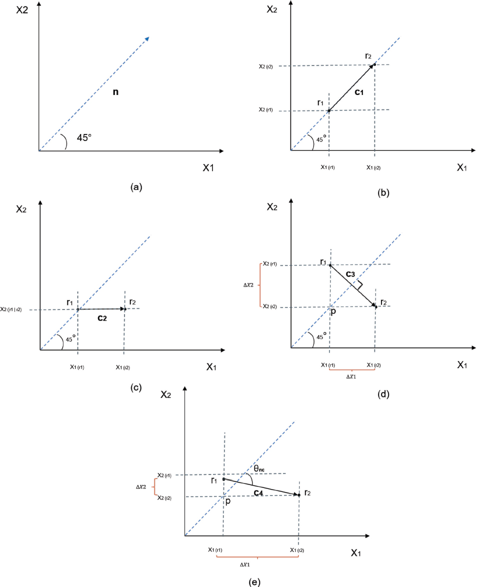
Figure 1.a – It shows only the vector n that is 45° from any of the axes that represent the magnitudes of the attributes. This direction of change represents the price gradient.

Figure 1.b – In this case (combination), there are two referents (r₁ and r₂) that are separated by a distance |c₁|. The distance separating r₁ and r₂ should correspond to a directly proportional change with respect to the prices of these referents, because in order to move the point from r₁ to r₂, both variables (X₁ and X₂) had to increase by equal magnitude. In other words, r₂ improves in every way over r1, and each variable contributes the same to the change. Here (X₂r₂ − X₂r₁/X₂r₂− X₂r₁) = 1

Figure 1.c – This case is similar to 1.b, but with the difference that the change between r₁ and r₂ consists of a variation only of the variable X₁, and since we assume that both variables contribute in the same way to the formation of the price, the impact we should expect on the price is half that compared to scenario 1.b.

Figure 1.d – A compensation scenario is shown here. Starting from point p, we must advance ∆X₁ horizontally to reach r₂, and move ∆X₂ vertically to obtain r₁. In this case ∆X₁= ∆X₂ and the angle formed by c and n is 90°. Again, if the variables have the same relative weight in the formation of the price, then neither referent has an advantage over the other, so the distance between them should not imply a difference in the prices of r₁ and r₂. In other words, if the relative importance assigned to the variables is correct, it follows that if there were a price difference between r₁ and r₂ it would not be attributable to X₁ and X₂.

Figure 1.e – Cases b, c and d show borderline situations. The case shown in figure 1.e is a general one, where the vector c forms any angle θnc with n.

The question now is how to incorporate what has been pointed out, into an operating model, and this is achieved by correcting the distance by cosine square of the angle between n and c, that is, by multiplying it by (cos θ_nc)².

The distance to be used (and to be corrected) is the Euclidean distance weighted by the relative importance of each of the variables. The distance between ri and rj will be

$$d_{ij}={[{\sum }_k {\alpha }_k{\left(X_{ik}-X_{jk}\right)}^2]}^{1/2} [8]$$

K is the number of variables.

The corrected distance will be of interest to the model

$$D{C}_{ij}=d_{ij}{[\cos {\theta }_{n\left(cij\right)}]}^2 [9]$$

The choice of cosine squared is obvious for three reasons: 1- a positive value for distance is preserved, 2 – it is consistent with the scenarios shown in figure 1: it worth one in the case of combination (1.b), it takes the value 1/2 in the intermediate situation 1.c, and 0 (zero) in the compensation situation (1.d), and 3 – the discount factor increases rapidly when the ability of the distance to explain the price difference decreases.

Now, the calculation to be programmed is simplified by considering the canonical to the origin of n, which has all coordinates with value 1 and $\mathbf{\left|}\mathit{n}\mathbf{\right|}\mathbf{=}\sqrt{\mathbf{k}}$.

The vector to the origin associated with the weighted distance between any two referents r₁ and r₂ is $<c_1,c_2,\dots ck>$ with the components shown in the equation (10)

$$c=<{\alpha }_1\left(r_{21}-r_{11}\right),{\alpha }_2\left(r_{22}-r_{12}\right),\dots {\alpha }_k\left(r_{2k}-r_{1k}\right)> [10]$$

Therefore $\mathit{n}\cdot \mathit{c}=\sum c_i$ and $\left|c\right|={[\sum c_i^2]}^{1/2}$.

3.3. The model to solve

What has been explained in sections 3.1 and 3.2 can be summarized as follows:

$$\mathit{\text{Min}}\sum \sum \left|{ϵ}_{ij}\right| [11]$$

s.t.

$$\sum {\alpha }_{\mathit{i}}\mathit{=}\mathit{1} [12]$$

$$D{C}_{ij}=d_{ij}{[\cos {\theta }_{n\left(cij\right)}]}^2 [13]$$

$$\cos {\theta }_{n\left(cij\right)}=\frac{\mathit{n}\cdot \mathit{c}}{\left|\mathit{n}\right|\cdot \left|\mathit{c}\right|} [14]$$

The joint determination of α and Φ by an iterative optimization procedure is then required, and it can be solved using any optimization program, we can even use Solver in Microsoft Excel.

3.4. Price estimation using the model

Section 3.3. describes the model for obtaining the vector of relative weights for the set of attributes and the proportionality constant but, does not indicate how these parameters obtained by this procedure can be used to give a price estimate of an interest asset.

There are at least two ways to use the weights obtained when applying the model presented:

3.4.1. Price that minimizes inconsistencies

This is a fairly obvious option, if we call r₀ the property whose price we wish to estimate (P₀), from equation (5) it follows that

$${ϵ}_{i0}=\left|\mathrm{\Delta }{P}_{i0}\right|-\mathrm{\Phi }D{C}_{i0} [15]$$

There will be as many new error terms as there are properties in the sample. The P₀ estimate we are looking for will be the value that minimizes the sum of the terms ϵ_i0 that is

$$P_0=\mathit{\text{argmin}}\sum \left|{ϵ}_{i0}\right| [16]$$

It should be noted that at this point the vector α is determined, so that the distances between the property in question and the comparables are also known, with P₀ being the only variable to be estimated.

3.4.2. Fitting a constant in a linear model

This option consists of assuming a linear model

$$P={\alpha }_1{X}_1+{\alpha }_2{X}_2+\cdots .+{\alpha }_n{X}_n+C [17]$$

In this case, the components of the vector a do not have to add one, but a condition is added, they must respect proportionality (relative importance) according to the vector α. That is, if for example α₁ is 1.5α₂, then in the same way a₁ is 1,5a₂ and so on. Then for [16] we simply search for C so that it minimizes the error within the sample.

In the next section, the results of both approaches will be presented on an example case. The procedure described is what we have called Method of the Corrected Distance (hereinafter MCD).

4. NUMERICAL EXAMPLE

In the examples for this article, we will consider that the determinants of value are intrinsic attributes of buildings, but that is only due to two simple reasons: the first is that to make the introductory application example simple, two explanatory variables have been taken; and secondly, the real cases presented in section 5 corresponds to apartments in the same commune, located in quite similar areas. In fact, the more similar the references in an appraisal are to each other and to the asset evaluated, the fewer variables and adjustments should be considered, contributing to the parsimony and simplicity of the procedures.

However, it is clarified that exogenous factors (from the environment) can play a relevant role in the value that the market assigns to a property. In fact, we find studies focused on the impact that can be attributed to a relevant factor linked to the dynamics and structure of the city; for example, noise (Szopinska et al., 2020; Aguirre & Ramos, 2005), road traffic (Guijarro, 2019), crime (Forys & Putek-Szelag, 2017), or subway lines (Sun et al, 2016; López-Morales et al, 2023); just to mention a few of the topics with recent research.

4.1. Calculation of the weights or relative importance of each variable

At this point we are going to work on a hypothetical case (Table 1) with only two variables or attributes (X₁ and X₂), and five referents (R₁ to R₅). In section 5 of the article, we will present a real and more robust example. This initial case serves to provide a simpler illustration.

To make practical sense of the variables, we will assume that we are talking about apartments, and X₁ is the floor number (height within the building) and X₂ is the common expenses in the building (expressed in the corresponding monetary unit).

We will also assume a market willing to pay more for high floors and less if it is a low floor (due to apprehensions about noise, insecurity, etc.). Similarly, high common expenses have a negative influence on the price. As indicated in section 3, the model requires that the relationship of the variables to the price be direct, so we convert the common expenses (ce) and the variable X₂ will actually express (1/ce) · 10³ - see Table 2 -.

The application of the MCD generates as a result α₁ = 0,228; α₂ = 0,772 and Φ = 6,245.

The model assigns greater weight to common expenses, although without discarding the height of the apartment. Of course, as in a regression model, these weights will depend on the units assigned to the different variables, they are factors that guarantee internal coherence in the model, they do not have an absolute interpretation.

4.2. Comparing the results with the Goal Programming method

Just to have a comparison with another method that objectively estimates the relative weights of the variables, we are going to calculate the results using Goal Programming (GP) - see Aznar & Guijarro (2007; 2012) for details of the model in this context -. GP works in a similar way to Linear Regression, but it is an optimization model where the hyperplane is obtained by minimizing a different loss function, without being subject to the same statistical assumptions, and being much less sensitive to the presence of outliers; in such a way that it has some advantages.

4.2.1. Estimation using “price that minimizes inconsistencies”

As an indicator of the degree of fit within the sample, we will use the well-known Mean Absolute Percentage Error (MAPE).

$$MAPE=\frac{1}{n}\sum \left|\frac{P_A-P_F}{P_A}\right| [18]$$

The MAPE for MCD is 2 %.

The application of the GP algorithm produces the result

$$p=47,125+1,250X_1+3,093X_2 [19]$$

And the result is a MAPE of 1.22%.

This is a performance indicator, but only within the sample that is used to calculate the parameters of each model. To appreciate how similar the results are outside the sample, we can compare the estimates with some contrast scenarios and that cover a wide range of possibilities: E₁ [X₁ = 1, X₂ = 1]; E₂ [X₁ = 4, X₂ = 5]; E₃ [X₁ = 20, X₂ = 1]; E₄ [X₁ = 15, X₂ = 5]; E₅ [X₁ = 5, X₂ = 15]; E₆ [X₁ = 1, X₂ = 20]; E₇ [X₁ = 20, X₂ = 10]; E₈ [X₁ = 10, X₂ = 20]; E₉ [X₁ = 20, X₂ = 20].

Table 3 shows the estimates of unit prices for nine apartments that have differences with respect to the two attributes considered in the example.

The same results are presented in Figure 2.

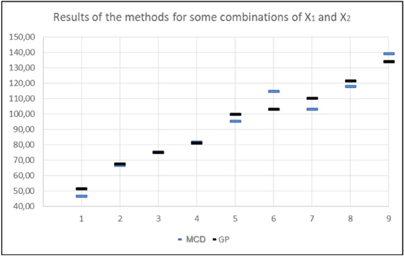
The results are similar in all cases, regardless of the level of the estimated price. Nor is there a bias in the sense that the estimate of one of the models is always above or below the estimate achieved by the other.

4.2.2. Estimation using fitting a constant in a linear model

This option yields a MAPE of 2.53%, and the results of the nine scenarios are those in Table 4.

Again, the data is presented graphically in figure 3.

The results are similar to the previous case, however, in this instance the difference with respect to GP is a little smaller than when the price that minimizes inconsistencies is used. However, although similar, the results are essentially different, as if they had been generated by completely different methods. Determining which of the two estimation approaches (price that minimizes inconsistencies or using fitting a constant in a linear model) could give better results in practice, it will require future tests with robust databases (additional cases to those presented here), where both the details of the properties and the price they reached on the market are also known.

Despite this, considering that the approach of fitting a constant actually requires determining several new parameters (all those present in equation 17), and that a linear structure is imposed, at least by a principle of parsimony, the option 3.4.1 which minimizes inconsistencies is preferable.

4.3. Performance of the method with respect to outliers

The method follows a similar behavior to GP also in terms of sensitivity to extreme values in some comparable, in general the results are not altered to a great extent when a data is varied.

As an example, the results of the original problem are compared below (Table 5), when the value of a property is estimated with X1 = 7 and X2 = 7, with respect to a modified scenario where the comparable 5 takes a price of 98 $ / m².

5. APPLICATION TO REAL DATA

The previous example served to show how the method works, but in this section, we will apply the procedure to data from specific properties, with more references and more variables to consider. First, we present an application to a set of purchase and sale transactions that have already been carried out, and then we focus on current offers available on the main real estate offering portal in Chile.

5.1. Real sales – cases available in the archives of the Santiago Real Estate Conservator

The information in Table 6 corresponds to the sale of ten apartments in the commune of Providencia, in the city of Santiago de Chile. All cases are apartments with two bedrooms and two bathrooms, of similar interior quality (at the time of sale), and which were sold in the last three years by a well-known real estate brokerage in the area. The details of the operations, as well as the architectural plans are public and available on the website of the Santiago Real Estate Conservator, and there are also details of the properties and operations on the websites: Avaluos (https://www.avaluos.cl/) and TocToc (https://www.toctoc.com/). Although the sales cover a considerable period of time, we have the advantage that for this group of properties all their characteristics are known in detail, including the price actually paid for each one.

Normally, bank appraisals with the purpose of guaranteeing a mortgage loan in Chile present only five or six market benchmarks; however, it has been decided to incorporate ten apartments to present the method.

Unlike the first example, these records correspond to actual transactions, and two new variables have been considered in the model: built area and age. The built area is made operational as the total equivalent area, which corresponds to the interior area plus half of the area corresponding to the balconies. On the other hand, and in response to the requirement of the model that the variables have a direct relationship with the price, the age is operationalized as the remaining useful life of the property, calculated as the difference between eighty years (useful life according to the tax office in Chile) minus age.

5.1.1. Results with MCD

The application of the MCD in this case generates as a result α₁ = 0,226; α₂ = 0,093; α₃ = 0,586; α₄ = 0,093; and Φ = 272,773.

The model assigns a clear prominence to X₃, followed by X₁, while X₂ and X₄, although considered relevant, have little relative weight.

Using price that minimizes inconsistencies, yields a MAPE of 2,80 % (Table 7).

5.1.2. Results with GP

The application of the GP algorithm produces the result

$$p=\mathrm{5,856}{X}_2+\mathrm{62,919}{X}_3+\mathrm{22,326}{X}_4 [20]$$

And the result is a MAPE of 2,80 % (Table 8).

Again, in this case with real market transactions, Method of the Corrected Distance achieves a performance very similar to those obtained by Goal Programming.

An important difference in this example is that GP completely overrides X1 and assigns almost all the importance to X₃ and X₄. Conversely, MCD is more eclectic maintaining all the variables. An additional example will help illustrate the point: if we want to evaluate an apartment whose explanatory variables are above the average of the sample, we expect an estimate of value that is also higher than the average, let us take the case of having X₁ = 9; X₂ = 7,14 (it is 190.000 for common expenses); X₃ = 88 and X₄ = 65. In this case, MCD generates an estimate of UF 7.088,53; while GP yields UF 7.048,84. Both estimates are unsurprisingly above the average value in the sample (UF 7.011), but MCD assigns a slightly higher value, partly because it is considering the effect of X₁.

5.2. Ads of apartments for sale from portalinmobiliario.com

From the midpoint between two emblematic parks in the eastern sector of the commune of Providencia in Santiago de Chile, and which corresponds to the intersection of Suecia and El Vergel streets, 10 referents were taken as close as possible to this intersection (Figure 4) and that in turn presented all the necessary information in the publication. All the dwellings correspond to 2-bedroom apartments, within a radius of 200 m. The area has homogeneous regulations, being a sector of buildings between 7 and 12 floors.

The details of each apartment are shown in Table 9.

5.2.1. Results with MCD

The application of the MCD in this case generates as a result α₁ = 0,206; α₂ = 0,281; α₃ = 0,427; α₄ = 0,085; and Φ = 445,668.

The built surface continues to have high relative importance, maintaining its position, as does the remaining useful life, which still holds the last place, although it remains important. The variable that has changed significantly is common expenses, acquiring greater weight within this sample. Finding some variation in the results compared to the real sales presented before is not at all strange, since there are differences in time, geography, and in the type of data itself (real sales versus offers).

Using price that minimizes inconsistencies, yields a MAPE of 3,74 %.

5.2.2. Results with GP

The application of the GP algorithm produces the result

$$p=\mathrm{373,272}{X}_1+\mathrm{117,894}{X}_2+\mathrm{59,395}{X}_3 [21]$$

And the result is a MAPE of 4,58 %.

In this case, MCD has achieved a lower MAPE than GP, although as already noted, that is not a definitive indicator of superiority of one method over another.

6. CONCLUSIONS

The article presents a novel valuation model, which operates under the premise of making the weights assigned to the factors that influence the value, manage to harmonize the price differences and the dissimilarities among the different properties that make up the sample of comparables.

The procedure is objective as far as possible, because once the variables of interest have been selected (process not covered in the methodology, but for which there are other techniques), the estimation is independent of the appraiser, and is based only on a nonlinear optimization program applied to the available data. Likewise, the examples presented show that the method generates consistent results, similar to those obtained by a proven methodology such as Goal Programming.

Regarding the daily professional practice of appraisal, using mathematical programming presents a disadvantage, as the procedure is more complex than other comparative methods (such as the traditional grid adjustment). This complexity demands a higher level of expertise from appraisers. However, for valuation professionals who are proficient in Optimization Methods, the Corrected Distance Method offers a valuable analytical tool that, as demonstrated by the examples provided, produces highly accurate estimates. Additionally, the model only needs to be programmed once in a flexible template, after which only the key variable values require adjustment. Thus, if the appraiser possesses the necessary skill, the Corrected Distance Method proves to be an objective, consistent and adaptable tool.

The work has focused on the residential property market within a well-defined geographical area, but there is an open invitation to evaluate its performance in other markets, such as offices, warehouses, land, etc. Furthermore, it may have applications beyond appraisals, and there is still work to be done to adapt it to estimates or forecasts in other areas. This is because it is essentially a generalizable method that estimates a response variable based on a set of explanatory variables, but it has been developed and presented within the framework of real estate valuation. Likewise, since the method is based on the internal coherence of the data in the sample, a modification could be worked on to assist in the detection of outliers. These lines of research remain open for further investigation.

CONFLICTS OF INTEREST

This research has not been funded by any company or institution. The author declares that there are no conflicts of interest.

FUNDING

This research has not received external funding.

REFERENCES

Aguirre Núñez, C. & Ramos Salinas, R. (2005). Impacto del Ruido Urbano en el Valor de los Departamentos Nuevos: un Estudio de Precio Hedónico Aplicado a Bienes Ambientales. Revista de la Construcción, 4(1), 59-69. https://www.redalyc.org/articulo.oa?id=127619365008

Agustin, K., Soewandi, H. & Widjojo, S. (2023). On the Weights for Characteristics and Comparables. Civil Engineering Dimension, 25(1). 37–47. https://doi.org/10.9744/ced.25.1.37-47

Aznar, J. & Guijarro, F. (2007). Estimating regression parameters with imprecise input data in an appraisal context. European Journal of Operational Research, 176(3), 1896–1907. https://doi.org/10.1016/j.ejor.2005.10.029

Aznar, J. & Guijarro, F. (2012). Nuevos métodos de valoración: modelos multicriterio. Universidad Politécnica de Valencia. España.

Coldwell, P., Cannaday, R. & Wu, C. (1983). The Analytical Foundations of Adjustment Grid Methods. Real Estate Economics, 11(1), 11–29.

Court, A. T. (1939). Hedonic price indexes with automotive examples, in ‘‘The Dynamics of Automobile Demand,’’ General Motors, New York, pp. 99-119

Forys, I. & Putek–Szelag. E. (2017). The Impact of Crime on Residential Property Value - On the Example of Szczecin. Real Estate Management and Valuation, 25(3), 51-61. https://doi.org/10.1515/remav-2017-0022

Grissom, T., Robinson, R. & Wang, K. (1987). A Matched Pairs Analysis Program in Compliance with FHLBB Memorandum R 418/C. The Appraisal Journal. 42-68.

Guijarro, F. (2013). Estadística aplicada a la valoración: Modelos multivariantes. Universidad Politécnica de Valencia. España.

Guijarro, F. (2019). Assessing the Impact of Road Traffic Externalities on Residential Price Values: A Case Study in Madrid, Spain. International Journal of Environmental Research and Public Health, 16(24), 5149. https://doi.org/10.3390/ijerph16245149

Guijarro, F. (2021). A mean-variance optimization approach for residential real estate valuation. Real Estate Management and Valuation, 29(3), 13-28. https://doi.org/10.2478/remav-2021-0018

Haas, G. C. (1922). A Statistical Analysis of Farm Sales in Blue Earth County, Minnesota, as a Basis for Farm Land Appraisal. Masters thesis, the University of Minnesota.

Isakson, H. R. (1986). The Nearest Neghbors Technique: An Alternative to the Ajustment Grid Method. AREUEA Journal 14(2), 274-286.

Kucharska-Stasiak, E. & Źróbek, S. (2015). An Attempt to Exemplify the Economic Principle in Real Property Valuation. Real Estate Management and Valuation, 23(3), 5-13. https://doi.org/10.1515/remav-2015-0020

López-Morales, E., Sanhueza, C., Herrera, N. & Espinoza, S. (2023). Land and housing price increases due to metro effect: An empirical analysis of Santiago, Chile, 2008–2019. Land Use Policy (132):106793 https://doi.org/10.1016/j.landusepol.2023.106793

Montgomery, D., Peck, E. & Vinig, G. (2002). Introducción al Análisis de Regresión Lineal. Compañía Editorial Continental. México.

Piracés, J. C. (2019). Tasación y mercado: Teoría y Práctica del Método Comparativo en la Tasación Inmobiliaria. Santiago de Chile.

Ratcliff, R. & Swan, D. (1972). Getting more from comparables by rating and regression. The Appraisal Journal, 68-75.

Sun, H., Wang, Y. & Li, Q. (2016). The Impact of Subway Lines on Residential Property Values in Tianjin: An Empirical Study Based on Hedonic Pricing Model. Discrete Dynamics in Nature and Society, ID 1478413, http://dx.doi.org/10.1155/2016/1478413

Szopinska, K., Krajewska, M. & Kwiecien, J. (2020). The Impact of Road Traffic Noise on Housing Prices – case study in Poland. Real Estate Management and Valuation, 28(2), 21–36. https://doi.org/10.1515/remav-2020-0013

Zaric, G. (n.d.). Quality Point. Found on https://professional.sauder.ubc.ca/re_creditprogram/course_resources/courses/content/330/qp_zaricreview.pdf

_______________________________

Autor de correspondencia: umcdip@gmail.com

¹ ORCID: https://orcid.org/0000-0001-7854-441X